In the market, it is crucial to spot the trend, but it is equally important to detect when the trend ends. Getting out of the trade is more difficult than entering the trade. In this blog, we will talk about one such technical indicator, the Parabolic SAR indicator, which helps in identifying when the trend ends.
The Parabolic SAR or Parabolic stop and reverse was developed by J. Welles Wilder. The Parabolic SAR is used by the traders to predict the direction of an asset as well as help in determining entry and exit points. In this article, we will go through the following points:
- Parabolic SAR calculation
- How to trade with Parabolic SAR
- Trading strategy with Parabolic SAR in Python
- Pros and cons of Parabolic SAR
The Parabolic SAR appears as a series of dots placed above or below the price mark as you can see in the chart.
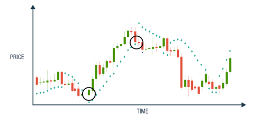
The dots above the price level is considered as a downtrend. Conversely, the dots below the price level is considered as an uptrend. The change in the direction of dots indicates the potential change in the price direction. For instance, you can observe at the start that the dots are below the price level. When it flips above the price, it could signal a further decline in price. The trend is strong when there is a wide gap between price and dots as you can observe at the end of the chart. In the sideways market, there is frequent interaction between price and dots.
Parabolic SAR calculation
The Parabolic SAR (PSAR) indicator uses:
- Extreme highest and lowest price in the current trend
- Acceleration factor: Acceleration factor determines the sensitivity of the Parabolic SAR.
Default setting
AF starts at 0.02 and increases by 0.02 each time the extreme point makes a new high/low. AF can reach a maximum of 0.2, no matter how long the trend extends.
Increasing the values of step and maximum step increases the sensitivity of the indicator, but it decreases its accuracy. Lowering the values of step and maximum step decrease the sensitivity of the indicator, but it improves its precision. We need to find a balance between these two values to generate quality signals. In our strategy, we will use values of (0.02,0.2)
Calculation of rising Parabolic SAR
Current SAR = Previous SAR + Previous AF(Previous EP – Previous SAR)
Where,
Previous SAR = Previous period SAR value
EP = Highest high of the current uptrend
AF = Acceleration factor
Calculation of falling Parabolic SAR
Current SAR = Previous SAR – Previous AF(Previous SAR – Previous EP)
where,
Previous SAR = Previous period SAR value
EP = Lowest low of the current downtrend
AF = Acceleration Factor
In our strategy, we will install and use the TA-Lib library (Python library for technical indicators) to calculate the Parabolic SAR values directly.
How to trade with the Parabolic SAR
Trending Market
The Parabolic SAR is best used when the market is trending; that is when the market has long rallies in either direction and have small corrections. It is advisable not to trade with the Parabolic SAR in a sideways market.
Higher time frames
If the time frame is small, Parabolic SAR will generate too many signals, and it might offer contradictory signals. On higher time frames, the trade will move slowly, and this will avoid false signals as most of the market noise is eliminated.
Better to use as an exit indicator
Parabolic SAR is used mostly as an exit indicator. Close buy position when price moves below the Parabolic SAR and close sell position when price moves above the Parabolic SAR. It also provides a stop loss level that moves closer to the market price regardless of the market direction.
Combine Parabolic SAR with other indicators
Parabolic SAR is a lagging indicator because it follows the price, and with the help of other indicators, we will be able to generate quality signals. It can be combined with many indicators. However, It is important to note that the role of Parabolic SAR is to determine the direction of trend and change in the direction of the trend. Combining Parabolic SAR with the other trend following indicator is not that useful as it will provide two trend confirmation signals. In the strategy, we are using Ichimoku indicator with the Parabolic SAR. To know more about Ichimoku cloud, you can refer to this link. Parabolic SAR can be used to determine optimal entry and exit points and Ichimoku cloud provide potential current and future support and resistance points.
Trading strategy with Parabolic SAR in Python
Now that you have an understanding of Parabolic SAR. Let’s implement the trading strategy in Python.
Import data
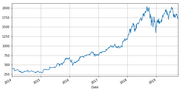
Importing Amazon (AMZN) data from 01-Jan-2014 to 01-Oct-2019. The data is imported from yahoo finance.
In [2]:
# Import pandas
import pandas as pd
# Import yfinance
import yfinance as yf
# Import data from yahoo finance
data = yf.download(tickers='AMZN', start='2014-01-01', end='2019-10-01')
# Drop the NaN values
data = data.dropna()
data.head()
[*********************100%***********************] 1 of 1 downloaded
Out[2]:
| Date | Open | High | Low | Close | Adj Close | Volume |
|---|---|---|---|---|---|---|
| 2013-12-31 | 394.58 | 398.83 | 393.80 | 398.79 | 398.79 | 1996500 |
| 2014-01-02 | 398.80 | 399.36 | 394.02 | 397.97 | 397.97 | 2137800 |
| 2014-01-03 | 398.29 | 402.71 | 396.22 | 396.44 | 396.44 | 2210200 |
| 2014-01-06 | 395.85 | 397.00 | 388.42 | 393.63 | 393.63 | 3170600 |
| 2014-01-07 | 395.04 | 398.47 | 394.29 | 398.03 | 398.03 | 1916000 |
In [4]:
# Import matplotlib
import matplotlib.pyplot as plt
plt.style.use('fast')
# Plot the closing price
data.Close.plot(figsize=(10,5))
plt.grid()
plt.show()
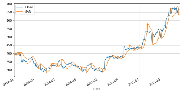
Parabolic SAR
Using SAR function from Ta-Lib library to calculate the parabolic. The input parameters are high price, low price, acceleration factor (AF), and maximum step.
As already discussed, acceleration factor increases by 0.02 each time the extreme point makes a new high/low, and it can reach a maximum of 0.2, no matter how long the uptrend/downtrend extends.
In [5]:
# Import talib
import talib
# Calculate parabolic sar
data['SAR'] = talib.SAR(data.High, data.Low, acceleration=0.02, maximum=0.2)
In [6]:
# Plot Parabolic SAR with close price
data[['Close', 'SAR']][:500].plot(figsize=(10,5))
plt.grid()
plt.show()
Ichimoku Cloud
The Ichimoku Cloud, also known as Ichimoku Kino Hyo consists of five plots and a cloud.
The default parameters of Ichimoku Cloud are 9, 26, 52, 26.
- Tenkan-sen (Conversion Line): (9-period high + 9-period low)/2
- Kijun-sen (Base Line): (26-period high + 26-period low)/2
- Senkou Span A (Leading Span A): (Tenkan-sen + Kijun-sen)/2
- Senkou Span B (Leading Span B): (52-period high + 52-period low)/2
- Chikou Span (Lagging Span): Close plotted 26 days in the past
In [7]:
# Calculate Tenkan-sen
high_9 = data.High.rolling(9).max()
low_9 = data.Low.rolling(9).min()
data['tenkan_sen_line'] = (high_9 + low_9) /2
# Calculate Kijun-sen
high_26 = data.High.rolling(26).max()
low_26 = data.Low.rolling(26).min()
data['kijun_sen_line'] = (high_26 + low_26) / 2
# Calculate Senkou Span A
data['senkou_spna_A'] = ((data.tenkan_sen_line + data.kijun_sen_line) / 2).shift(26)
# Calculate Senkou Span B
high_52 = data.High.rolling(52).max()
low_52 = data.High.rolling(52).min()
data['senkou_spna_B'] = ((high_52 + low_52) / 2).shift(26)
# Calculate Chikou Span B
data['chikou_span'] = data.Close.shift(-26)
In [8]:
data.head()
Out[8]:
| Date | Open | High | Low | Close | Adj Close | Volume | SAR | tenkan_sen_line | kijun_sen_line | senkou_spna_A | senkou_spna_B | chikou_span |
|---|---|---|---|---|---|---|---|---|---|---|---|---|
| 2013-12-31 | 394.58 | 398.83 | 393.80 | 398.79 | 398.79 | 1996500 | NaN | NaN | NaN | NaN | NaN | 361.08 |
| 2014-01-02 | 398.80 | 399.36 | 394.02 | 397.97 | 397.97 | 2137800 | 393.8000 | NaN | NaN | NaN | NaN | 360.87 |
| 2014-01-03 | 398.29 | 402.71 | 396.22 | 396.44 | 396.44 | 2210200 | 393.9112 | NaN | NaN | NaN | NaN | 361.79 |
| 2014-01-06 | 395.85 | 397.00 | 388.42 | 393.63 | 393.63 | 3170600 | 402.7100 | NaN | NaN | NaN | NaN | 349.25 |
| 2014-01-07 | 395.04 | 398.47 | 394.29 | 398.03 | 398.03 | 1916000 | 402.7100 | NaN | NaN | NaN | NaN | 357.20 |
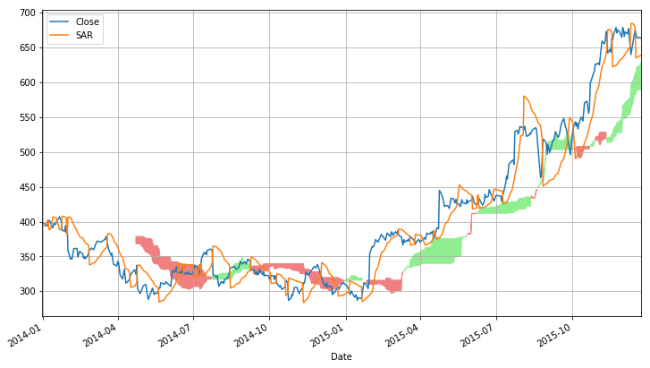
Plot komu Cloud
Komu cloud is a space between Senkou Span A and Senkou Span B. The cloud edges provide potential current and future support and resistance points. We are plotting komu cloud with the closing price and parabolic SAR. We plot cloud in light green when Senko span A is greater than Senko span B. We plot cloud in light coral when Senko span B is greater than Senko span A.
In [9]:
# Plot closing price and parabolic SAR
komu_cloud = data[['Close','SAR']][:500].plot(figsize=(12, 7))
# Plot Komu cloud
komu_cloud.fill_between(data.index[:500], data.senkou_spna_A[:500], data.senkou_spna_B[:500],
 where=data.senkou_spna_A[:500] >= data.senkou_spna_B[:500], color='lightgreen')
komu_cloud.fill_between(data.index[:500], data.senkou_spna_A[:500], data.senkou_spna_B[:500],
 where=data.senkou_spna_A[:500] < data.senkou_spna_B[:500], color='lightcoral')
plt.grid()
plt.legend()
plt.show()
Buy Signal
We take the buy position when the price is above the Komu cloud and parabolic SAR is below the price.
In [10]:
data['signal'] = 0
data.loc[(data.Close > data.senkou_spna_A) & (data.Close >
 data.senkou_spna_B) & (data.Close > data.SAR), 'signal'] = 1
Sell Signal
We sell when the price is below the Komu cloud and parabolic SAR is above the price.
In [11]:
data.loc[(data.Close < data.senkou_spna_A) & (data.Close <
 data.senkou_spna_B) & (data.Close < data.SAR), 'signal'] = -1
In [12]:
data['signal'].value_counts()
Out[12]:
 0 1037
 1 270
-1 140
Name: signal, dtype: int64
Calculate Strategy Returns
We calculate the daily returns. Then we calculate strategy returns by multiplying the daily returns with the previous day signal. Further we calculate the cumulative product of the strategy returns.
In [13]:
# Calculate daily returns
daily_returns = data.Close.pct_change()
# Calculate strategy returns
strategy_returns = daily_returns *data['signal'].shift(1)
In [14]:
# Calculate cumulative returns
(strategy_returns+1).cumprod().plot(figsize=(10,5))
# Plot the strategy returns
plt.xlabel('Date')
plt.ylabel('Strategy Returns (%)')
plt.grid()
plt.show()
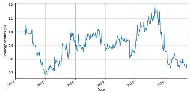
Summary of the trading strategy
This is a straightforward strategy based on parabolic SAR and Ichimoku cloud. However, it generates good returns for over 5 years. But there are things which you need to take care during backtesting such as stop-loss, slippage. Now it’s your turn to tweak the code and make it more close to the live environment.
Pros and cons of Parabolic SAR
The advantage of the Parabolic SAR is that it works best when there is a strong trend in the market. Also, in comparison to other trend indicators, it provides better exit signals. The major drawback is that when there is no trend or market is choppy, the dotted lines of Parabolic SAR continuously turnaround above or below the price. This is mostly lead to false signals.
Conclusion
Thus, we have seen how to calculate Parabolic SAR as well as its application in trading. We have also understood the advantages and disadvantages of the Parabolic SAR indicator
Do let us know if you loved the article and any other feedback in the comments below.
You can learn more about technical indicators and build your own trading strategies by enrolling in the Quantitative Trading Strategies and Models course on Quantra.
If you want to learn various aspects of Algorithmic trading then check out our Executive Programme in Algorithmic Trading (EPAT®). The course covers training modules like Statistics & Econometrics, Financial Computing & Technology, and Algorithmic & Quantitative Trading. EPAT® is designed to equip you with the right skill sets to be a successful trader. Enroll now!
Disclaimer: All data and information provided in this article are for informational purposes only. QuantInsti® makes no representations as to accuracy, completeness, currentness, suitability, or validity of any information in this article and will not be liable for any errors, omissions, or delays in this information or any losses, injuries, or damages arising from its display or use. All information is provided on an as-is basis.
ref: https://blog.quantinsti.com/parabolic-sar/